Rare Event Detection and Analysis in Flow Cytometry Protocol

Introduction of Rare Event Detection and Analysis in FC

This chapter will detail the flow cytometric identification and quantification of three rare populations: one in liquid tissue (mesenchymal stem cells in a bone marrow aspirate), one that exists as aggregates in suspension (breast cancer stem/progenitor cells in pleural effusion), and one in solid tissue (pericytes in disaggregated adipose). Detailed protocols will be given for preparation of single cell suspensions from these sources. This will be followed by instructions for efficient staining with multiple antibodies, sample acquisition, and data analysis.

Methods of Rare Event Detection and Analysis in FC

Preparation of Single Cell Suspensions

Bone Marrow

Bone marrow is usually obtained by aspiration from the posterior iliac crests. It can also be obtained from discarded surgical specimens (femoral head in hip replacements, rib section in lung lobectomy, or from cadaveric vertebrae. Bone marrow should be aspirated into heparinized syringes (sodium heparin, 10 U/mL) and held at ambient (not refrigerated) temperature.

1. Bone marrow mononuclear cells, depleted of mature erythrocytes and mature granulocytes, are prepared by Ficoll/ Hypaque gradient centrifugation.
2. Dilute aspirated bone marrow or bone marrow flushed from bones to 30 mL with PBS–0.1% albumin (see Note 3). The total number of cells per tube should not exceed 50×10⁶.
3. Pipette 15 mL of Ficoll/Hypaque into a 50 mL polypropylene conical tube.
4. Using a 10 mL pipette, carefully layer 30 mL of diluted bone marrow over the Ficoll/Hypaque (see Note 4). Set centrifuge to 25°C, and spin at 400×g for 45 min (brake off).
5. After centrifugation, aspirate and discard the upper layer (diluent) with a 10 mL pipette (see Note 5).
6. Using a 10-mL pipette, carefully collect the Buffy Coat and pipette into a new 50-mL conical tube (see Note 6).
7. Wash the Buffy Coat twice with 50 mL of PBS–0.1% albumin (400×g, 7 min, 25°C).
8. Resuspend in 2 mL of PBS–0.1% albumin and hold on ice.
9. Count cells and record cell concentration and volume (see Note 7).

Malignant Pleural Effusions

Pleural effusions are collected into plastic containers by suction. Ideally they should be heparinized (sodium heparin, 10 U/mL) because they often contain serous fluid capable of clotting. They contain cells in suspension, but tumor is usually in clumps that range from microscopic to visible. The cell count and volume vary considerably from sample to sample (see Note 8).

1. Record the volume and cell count of the unmanipulated sample (see Note 9).
2. Concentrate the cells and cell clumps by centrifugation (400×g, 7 min, 4°C).
3. Discard supernatant and resuspend the pellet in 10 mL Collagenase type I/DNase solution (see Note 10).
4. Place sample in a shaking waterbath (e.g. Bellydancer) at 37°C for 30 min, maximum agitation setting.
5. Place a 70 mm cell strainer in the mouth of a new labeled 50 mL conical tube.
6. Using a 10 mL pipette, transfer material from the collagenase digestion tube into the cell strainer.
7. Add 10 mL of PBS–0.1% albumin to the digestion tube and transfer any remaining material to the cell strainer. Discard strainer.
8. Bring volume of strained cells to 50 mL with PBS–0.1% albumin, centrifuge at 400×g for 7 min, 4°C and discard supernatant.
9. Add 45 mL of NH4Cl lysing solution and mix (see Note 11).
10. Centrifuge at 400×g, 4°C for 10 min.
11. Pour off the supernatant and loosen cell pellet.
12. Resuspend in 2 mL of PBS–0.1% albumin and hold on ice.
13. Count cells on a hemacytometer.

Whole Adipose Tissue

1. Adipose tissue is a byproduct of aesthetic surgery. It may be removed in the form of solid tissue or lipoaspirate. This protocol assumes solid adipose tissue. The expected yield of stromal/ vascular cells is approximately 1×10⁶ cells/g of tissue. 1. Record the weight of adipose tissue.
2. Cut the tissue in large pieces using the sterile scissors and distribute into 50 mL conicals (approximately 10 g of fat per tube).
3. Thoroughly mince tissue in the 50 mL conical tubes using scissors.
4. Add 30 mL of Collagenase type II solution per tube.
5. Vortex the conical tube and incubate at 37°C in a shaking water bath for 15 min, maximal agitation.
6. Examine the tubes to estimate efficient digestion. The presence of excessive clumps indicates under-digestion. The appearance of a clear yellow lipid layer indicates over-digestion. Reincubate in the water bath if full digestion is not achieved. Repeat every 5 min for a maximum of 30 min total digestion time.
7. Add 10 mL of EDTA buffer to neutralize ongoing collagenase activity.
8. Centrifuge at 400×g for 10 min at 25°C.
9. Collect all semi-solid top fat layers from all tubes into 50 mL polypropylene conical tubes. Add 30–40 mL of PBS–0.1% albumin and shake thoroughly to homogenize (see Note 12).
10. Vortex the remaining contents of the digestion conical tubes and pass the contents through the 425 mm and 180 mm large sterile sieves into the 1,000 mL Nalgene jar. Use a glass pestle if necessary.
11. Wash the sieves with up to 100 mL of PBS–0.1% albumin.
12. Collect the sieved sample from the basin to 50 mL or 200 mL conical tubes.
13. Add the diluted fat from the top layer of the digest to the sieves and pass through using the glass pestle.
14. Centrifuge the sieved cells at 400×g for 7 min at 4°C.
15. Discard supernatant and combine all cell pellets in one to two 50-mL conical tubes.
16. Wash the cells with PBS–0.1% albumin (50 mL per tube).
17. Centrifuge at 400×g for 7 min at 25°C.
18. Discard supernatant and loosen the cell pellet.
19. Add 45 mL of NH4 Cl lysing solution per tube and mix.
20. Centrifuge at 400×g, 4°C for 10 min.
21. Pour off the supernatant and loosen cell pellet.
22. Resuspend in 2 mL of PBS–0.1% albumin and hold on ice.
23. Count cells on a hemacytometer.

Surface Staining

1. Pellet cells at 400×g for 10 min at 4°C. Discard supernatant (see Note 13).
2. Resuspend cell pellet in 5 mL of neat decomplemented (56°C, 30 min) mouse serum (see Note 14).
3. Pellet cells (400×g, 10 min, 25°C) and aspirate the supernatant as thoroughly as possible without disturbing the pellet (see Note 15).
4. Stain the dry pellet for surface markers by the addition of 2 mL of each monoclonal antibody (see Note 16).
5. Add antibodies in the following order (see Note 17):
• Bone marrow mesenchymal cells
• CD105-FITC
• CD73-PE
• CD34-ECD
• CD90-PC5
• CD117-PC7
• CD31-APC or CD133-APC
• CD45-APC-Cy7
• Pleural fluid
• CD44-PE
• CD90-biotin-streptavidin-ECD
• Lineage cocktail: CD14-PC5, CD33-PC5, and Glycophorin A-PE-Cy5.
• CD133-APC
• CD117-PC7
• CD45-APC-Cy7
• Adipose pericytes
• CD3-FITC
• CD146-PE
• CD34-ECD
• CD90-PC5
• CD117-PC7
• CD31-APC
• CD45-APC-Cy7
6. Incubate for 30 min on ice in the dark.
7. Dilute surface stained cell pellets in 1 mL of staining buffer.
8. Centrifuge at 400×g for 7 min at 25°C.
9. Discard supernatant and loosen the cell pellet.

Intracellular Staining

Staining for intracellular antigens requires fixation and permeabilization, and is usually performed after surface staining.

• Following surface staining, pellet cells at 400×g for 10 min at 4°C. Discard supernatant with care to create a dry pellet.
• Fix stained cells for 20 min at ambient temperature with 200 mL of PBS and 200 mL of 4% methanol-free formaldehyde in hypertonic PBS-A (see Note 18).
• Centrifuge at 400×g for 7 min at 25°C.
• Discard supernatant with care to create a dry pellet and flick to loosen.
• Permeabilize fixed cells by addition of 200 mL of permeabilization solution containing saponin (10 min at ambient temperature).
• Intracellular cytokeratin staining of pleural effusion cells:
• Centrifuge at 400×g for 7 min at 25°C.
• Decant supernatant with care to create a dry pellet and flick to loosen.
• Add 5 mL of neat mouse serum to cell pellet, incubate at ambient temperature for 5 min, centrifuge, and decant to dry pellet.
• Loosen cell pellet and add 2 mL of anti-pan cytokeratin-FITC for 30 min.
• Dilute cytokeratin stained cell pellets in 500 mL of staining medium.
• Centrifuge at 400×g for 7 min at 25°C and discard supernatant to a dry pellet.
• Loosen cell pellets and dilute to a cell concentration of ten million cells/400 mL (25×10⁶ /mL) of staining buffer.
• Transfer to 12×75 mm tubes with 35 mm filter caps for flow cytometry.
• DNA content by DAPI staining for bone marrow mesenchy mal cells, adipose pericytes, and pleural effusion cells:
• Disaggregate cell pellets and dilute to a cell concentration of ten million cells/400 mL of staining buffer.
• Add 16 mL of DAPI stock solution to a final concentration of 8 mg/mL (see Note 19).
• Transfer to 12×75 mm tubes with 35 mm filter caps for flow cytometry.

Instrument Setup and Standards

IgG Capture Bead Staining

1. Vortex CompBeads thoroughly before use (see Note 20).
2. Label a separate 1.5 mL Eppendorf tube for each mouse monoclonal antibody conjugated to a tandem dye (e.g. ECD, PE-Cy5, PE-Cy7, and APC-Cy7).
3. Add one full drop (approximately 60 mL) of anti-mouse Ig CompBeads to each Eppendorf tube.
4. Centrifuge for 10 min at 400×g. Carefully aspirate supernatant to ensure a “dry pellet” (see Note 21).
5. Sonicate each tube for 10 s in a water bath sonicator (see Note 22).
6. Add 2 mL of each antibody directly to beads (one antibody per tube) and gently reflux.
7. Incubate for 15 min at room temperature in the dark (see Note 16).
8. Add 1 mL of mouse serum and incubate for 5 min at room temperature (see Note 23).
9. Add 100 mL of staining buffer and reflux.
10. Sonicate each tube for 10 s.
11. Add 1 mL of staining buffer. For manual compensation, add one drop of negative CompBeads to each test tube that contains antibody stained beads (see Note 24).
12. Centrifuge beads for 10 min at 400×g, decant and carefully blot to remove residual supernatant (see Note 25).
13. Resuspend washed beads in 0.5 mL of staining buffer.
14. Transfer to 12×75 mm snap cap tubes for flow cytometry.
15. Sonicate for 10 s prior to acquisition on the flow cytometer.

Instrument Setup and Sample Acquisition

These protocols have been validated on Beckman Coulter CyAn and Gallios cytometers. This protocol is applicable to all cytometers equipped with a UV or violet laser, a blue laser, and a red laser.

1. The cytometer is calibrated to predetermined photomultiplier target channels prior to each use using SpectrAlign beads and 8-peak Rainbow Calibration Particles (see Note 26).
2. The data from 8-peak beads can also be used to monitor instrument sensitivity (resolution of dim peaks) and instrument linearity.
3. All fluorescence parameters are collected in the logarithmic mode, with the exception of DAPI emission at 455 nm which is collected in the linear mode (see Note 27).
4. Acquire unstained cells or beads first, and then each single stained sample (bead or cells) from the shortest emission wavelength (FITC) to the longest (e.g. CD45-APC-Cy7).
5. Run a rinse tube. Then run analytical samples with a rinse tube in between if needed (see Note 28). Do not apply spectral compensation. This will be done offline with analytical software.

How Many Events to Acquire

Not everything that is detected by a flow cytometer is a cell. In fact, in messy samples like disaggregated solid tissues, cells are sometimes in the minority. Rare event problems sometimes necessitate the acquisition of millions of events in order to obtain the required number of cells. The correct number depends on three factors: (1)The proportion of cells to debris; (2) The signal-to-noise ratio of the population of interest compared to all other events; (3) The frequency of the population of interest.

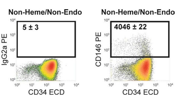Figure 1. Estimation of the lower limit of detection from an isotype control.

Discriminating between genuine events and potential sources of artifact such as debris will be illustrated in each example. The inclusion of dead or dying cells, autofluorescent events, or subcellular debris distorts both the numerator (population of interest) and denominator, and makes for an unreliable analysis. Much of the literature dealing with flow cytometry of cultured or disaggregated cells suffers to a greater or lesser extent from inclusion of such sources of artifact.

The signal-to-noise ratio encompasses both the distance (in fluorescence or scatter intensity) between positive and negative populations, and the variability (spread) of those populations in multiparameter space. Isotype controls or other definitive negative populations are often helpful to determine the boundaries defining a population of interest. Even when positive and negative populations appear to be well separated, acquisition of millions of events often reveals a scattering of false positive events within the multiparameter space of the population of interest. Creative gating, including elimination of sources of artifact and use of multiple parameters (both positive and negative) to define the population of interest, can often increase the signal-to-noise ratio. Ultimately, the frequency of false positive events determines the lower limit of detection and thus the maximum number of cells to be acquired. By performing replicate determinations, we were able to calculate the 95th percentile of the false positive event frequency is 0.0085% or 1 event in 11,790. Since acquiring 100 events of a population of interest is sufficient to give a CV of 10%, acquiring 1,179,000 events will take the assay to its limit of sensitivity, and acquiring more cells will do nothing to improve the result.

As expected, the number of positive events increases linearly with the number of events acquired and the variability between triplicate frequency estimates (Percent positive) decreases. Importantly, the measured coefficient of variation (CV, calculated as the standard deviation/mean) of the triplicate determinations decreases markedly. This empirical demonstration also shows the adequacy of the CV determined by a simpler alternative approach, Poisson statistics. Poisson statistics deal with the probability distribution of rare events. The Poisson CV of the counting error, defined as 100/√positive events counted, is 10% when 100 events are counted. In this example, the frequency of positive events (0.04%) requires that 250,000 events be acquired to achieve a CV of 10%.

There is one more aspect of signal-to-noise that counting statistics do not take into account, and that is the distribution of the population of interest in multiparameter space. Given the knowledge that T-cells are very constrained with respect to the range of CD3 and CD45 expression, very low numbers of positive events (in this case 23 CD3+ events, Poisson CV=20.9%) can be reliably detected.

Data Analysis of Three Examples: Bone Marrow Mesenchymal Stem Cells, Cytokeratin+Cells in a Malignant Pleural Effusion, and Pericytes in Human Adipose Tissue

We perform spectral compensation and data analysis offline, using VenturiOne or Kaluza software both of which have been designed to accommodate very large datafiles. After creating compensation matrices using the data from our single-stained beads, we create a playlist of datafiles in which each datafile is associated with an analysis template and a compensation matrix. Arriving at an adequate analysis template is an iterative process that used to be quite painful. The use of playlists to organize datafiles and compensation files from different directories, and the ability to export results to spreadsheets greatly facilitates reanalysis and revisiting data sets with new questions. Our analysis strategy usually proceeds in three steps:

1. First we eliminate sources of interference with logical gates. These may include event bursts (from transient fluidic disturbances), cell–cell doublets and clusters, subcellular debris, dead cells, and autofluorescent events.
2. Next, we decide on our classifier parameters. These are used to define the major population(s) of interest.
3. Next outcome parameters to be measured on each classifier population are determined. The distinction between classifier and outcome parameters is sometimes clear, but sometimes it is quite fluid, especially when exploring a new combination of analytes. At this stage it is often helpful to color-event cells positive for the outcome parameters and examine their expres sion on plots of the classifier parameters.

Elimination of Sources of Interference

Interference can come from many sources including fluidic disturbances, nonspecific binding of antibodies (dead and dying cells are adept at this), and cells with intrinsic autofluorescence (particularly cultured cells and some populations from fresh disaggregated tissues).

1. Fluidic disturbances alter laminar flow within the flow cell and results in increased variability in measurements, particularly light scatter. It is easy to spot transient fluidic disturbances by plotting a time parameter (or event count) versus log side scatter. Such a disturbance can be seen in the pleural effusion example. These events can be examined in isolation and removed from the analysis with a logical gate, if they prove to have altered marker expression.
2. Cell doublets and clusters, resulting from physical aggregation or coincidence are also problematic when large numbers of events are acquired. For DNA analysis, a doublet appears as a single cell with 4N DNA. For phenotypic analysis a T-cell/B-cell conjugate looks like a single cell with coexpression of T- and B-cell markers. Clusters are easily removed by pulse analysis of the triggering parameter. In our examples, we compare forward scatter pulse height (labeled FS lin) to forward scatter pulse width (labeled Pulse width) and eliminate event clusters that are too wide (i.e. have too long a time of flight) for their pulse height. In our examples the frequency of clusters ranges from 5% to 26%.
3. Dead and dying cells may also have altered marker expression, so it is always desirable to eliminate them from the analysis. This can be approached in several ways. In all of the examples given here, cells were permeabilized after staining and fixation in order to facilitate DAPI staining of cellular DNA. This has two benefits: (1) subcellular debris and hypodiploid (apoptotic) cells are easily identified and removed on a plot of DAPI log fluorescence intensity versus FS; (2) display of DAPI fluorescence on a linear scale provides a low-resolution cell-cycle analysis (see Notes 29 and 30). In our adipose example, 14% of events, most of them subcellular debris resulting from tissue digestion, had<2N DNA. Even after limiting the analysis to cells with DNA content ³2N, early apoptotic events with intact DNA may still be present. These can be identified and eliminated by their characteristic light scatter profile (generally low forward scatter with too much side scatter relative to forward scatter). In our adipose example the T-cell marker CD3 was used as a “Dump Gate” and CD3+ T cells were color evented and backgated on the light scatter plot. This gives us a point of reference to eliminate events with lower forward light scatter. This method assumes that the cells of interest have at least as high light scatter as small resting T-cells (see Note 31).
4. Elimination of events with saturating fluorescence. It is highly desirable to adjust PMT gains such that all positive events are on scale. In rare cases this is not possible without unbalancing PMT gain or obscuring dim positive events. Although this is a relatively small proportion of events, they must be removed from the analysis. Because their fluorescence is unknown, they cannot be spectrally compensated and will appear positive in the adjacent PE channel.
5. Cellular autofluorescence results from expression of naturally fluorescent biomolecules such as flavinoids. Autofluorescence can be distinguished from fluorescence specific to most of the dyes used in cytometry by it’s broad emission spectrum. Autofluorescent biomolecules are often excited better with short wavelength light than with long wave lengths. If the cell population of interest is autofluorescent, one is generally limited to long excitation wavelengths (e.g. red diode laser). In our examples, mesenchymal stem cells, adipose pericytes, and cytokeratin+breast cancer cells, the cells of interest are not autofluorescent, so we can use compound logical gates to eliminate events that excite with 488 nm light and emit in the ranges detected by FL1, FL2, and FL3 channels (e.g. using 530/30, 584/42, and 675/20 bandpass filters, respectively). In the pleural effusion example, relatively few events fall within all three diagonal gates, and these are uniformly cells with high light scatter.
6. Nonspecific fluorescence (autofluorescent or caused by nonspecific antibody binding) can be eliminated using a dump gate, that is, a marker which the population of interest is known not to express. If the dump gate uses a dye such as FITC, which is within the range of autofluorescent emission, it eliminates cells binding the antibody specifically and nonspecifically, and autofluorescent events as well. Nonspecific antibody binding is also minimized by a preincubation/blocking step with normal mouse serum prior to staining.

Identification of Classifier Parameters

Classifier parameters are those used to identify populations of interest. Thinking of parameters as either primary or secondary markers, or outcomes creates a hierarchical model, focuses the analysis, and eliminates the “all possible combinations” problem encountered in multi-parameter analysis.

1. Primary classifiers can be strung together as a Boolean AND gate.
2. Secondary classifiers branch into multiple populations of interest.

Measurement of Outcome Parameters on Populations Identified by Classifiers

The division between classifiers and outcomes is not rigid and often depends on how one frames a biologic question. For example, do we wish to start with cells that secrete interferon gamma (classifier) and examine lymphocyte subsets as outcomes, or wish to define lymphocyte subsets (classifiers) and determine (as out-comes) the proportion of cells secreting interferon gamma in each? As such, outcomes are final branch points in our hierarchical mode.

Browse by Primary Antibodies

Browse by Secondary Antibodies

Browse by Control Antibodies