Flow Cytometric FRET Analysis of Protein Interaction Protocol

Overview

Introduction of Flow Cytometric FRET Analysis

Modern biochemistry and molecular biology have served to identify hundreds of pairs of cellular proteins that are in vitro capable of interacting with each other. These protein–protein interactions are crucial in both maintaining the stable "resting" state of cells and in driving activation processes that allow cells to respond to external stimuli. Hence it becomes more and more important to be able to detect such interactions in situ inside or on the surface of cells. Fluorescence techniques are widely used to quantify molecular parameters of various biochemical and biological processes in vivo because of their inherent sensitivity, specificity, and temporal resolution. Combination of fluorescence spectroscopy with flow cytometry provided a solid basis of rapid and continuous improvements of these technologies. A major asset in studying molecular level interactions was the application of fluorescence resonance energy transfer (FRET) to cellular systems. Applying fluorescent-labeled antibodies, proteins, lipids, or other biomolecules either using organic dyes or fluorescent fusion proteins, the FRET technique can be used to determine inter- and intramolecular distances of cell surface components in biological membranes, as well as molecular associations inside live or intact cells. Excellent reviews are available on the applicability of FRET to biological systems as well as descriptions and comparison of various approaches. Only a few are quoted here.

FRET is a special phenomenon in fluorescence spectroscopy during which energy is nonradiatively transferred from an excited donor molecule to an acceptor molecule. For the process to occur, a set of conditions have to be fulfilled:

1. The emission spectrum of the donor has to overlap with the excitation spectrum of the acceptor. The larger the overlap, the higher the rate of FRET is.

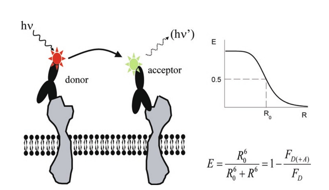Figure 1. FRET basics.

2. The emission dipole vector of the donor and the absorption dipole vector of the acceptor need to be close to parallel. The rate of FRET decreases as the angle between the two vectors increases. In biological situations where molecules are free to move (rotate), we generally assume that dynamic averaging takes place, i.e., the donor and the acceptor assume many possible steric positions during the excited-state lifetime of the donor, among them positions that can yield an effective transfer of energy. There are cases when the aforementioned assumption of dynamic averaging is most likely correct (e.g., antibodies labeled by fluorescent dyes bound to the antibody via flexible linkers); however, in some cases, it is certainly incorrect (e.g., fluorescent dyes intercalated into DNA). FRET taking place between proteins tagged by GFP (green fluorescent protein) or its derivatives represents an intermediate case in which the assumption of dynamic averaging is a relatively good approximation.

3. The distance between the donor and acceptor should be between 1 and 10nm.

This latter phenomenon is the basis of the popularity of FRET in biology: The distance over which FRET occurs is small enough to characterize the proximity of possibly interacting molecules; under special circumstances, it even provides quantitative data on exact distances and, additionally, information on the spatial orientation of molecules or their domains. Hence the very apropos term from Stryer, who equaled FRET to a "spectroscopic ruler". The usual term for characterizing the efficiency of FRET is E, which is the ratio of excited-state donor molecules relaxing by FRET to the total number of excited donors. The rate of the energy transfer process is dependent on the negative sixth power of the distance between the donor and the acceptor, resulting in a sharply dropping curve, practically eliminating FRET above a separation of 10 nm for the usual fluorophores. Conversely, as the distance reaches values below 1 nm, strong ground-state interactions or transfer by exchange interactions become dominant at the expense of FRET.

The occurrence of FRET has profound consequences on the fluorescence properties of both the donor and the acceptor. An additional de-excitation process is introduced in the donor, which decreases the fluorescence lifetime and the quantum efficiency of the donor, rendering it less fluorescent. The decrease in donor fluorescence (often termed donor quenching) can be one of the most facilely measured spectroscopic characteristics that indicates the occurrence of FRET. Additionally, since the acceptor is excited as a result of FRET, those acceptors that are fluorescent will emit photons (proportional to their quantum efficiency) also when FRET occurs. This is called sensitized emission and can also be a good measure of FRET.

Flow cytometric FRET (FCET) methods that can be implemented on commercial flow cytometers exploit one or both of these phenomena. The main advantage of the flow cytometric approach is the ability to examine large cell populations in a short time, and still provide FRET efficiency values up to single-cell resolution (albeit averaged over each cell). In a simplified scenario, population averages from the flow cytometer can be used to estimate an overall FRET efficiency for the whole cell population measured. While in theory there are at least 22 different possible approaches to quantifying FRET, some of these have never been tested, and many require a (usually microscope-based) system where cells or their compartments can be revisited once or several times for completing the measurement. Among the eight approaches applicable to flow cytometry, most require extensive modification of the equipment. Most of these methods are based on the measurement of conventional hetero-FRET in which spectroscopically different donor and acceptor molecules interact with each other. However, there is another modality of FRET interactions which takes place between identical fluorophores, i.e., the donor and acceptor molecules are of the same kind. The only manifestation of the phenomenon called homo-FRET is the decreased fluorescence anisotropy of the fluorophore population. Although instruments capable of recording polarized fluorescence intensities do not abound, the measurement of homo FRET makes quantitative analysis of large-scale protein clusters possible, since the fluorescence anisotropy changes inversely with the average number of proteins in a cluster. The approaches discussed in this chapter are based on hetero-FRET; the simple donor quenching-based FCET method and the more complex, but fully quantitative ratiometric, intensity-based FCET have already been extensively and successfully applied to biological systems. Finally, we shall describe a modification of the latter approach that allows a cell-by-cell correction for autofluorescence and thus can reduce the uncertainty of the quantitative determination of FRET when fluorescence signals are low. The necessary mathematical details will be introduced along with the measurement procedure, so that the importance and utility of the various control samples can be fully appreciated.

Materials of Flow Cytometric FRET Analysis

Cellular Systems

The easiest targets of FCET measurements are cells growing in suspension, such as those of lymphoid origin that can directly be labeled in suspension.
Cells that grow attached to substratum need to be trypsinized. Use a trypsin–EDTA solution that is appropriate for the cell line examined. Usually, 0.05% w/v trypsin and 2 mM EDTA work well, but cells that have spent a longer time in the same culture dish or express a massive extracellular matrix may need a more vigorous treatment. In our experience, a 5-min trypsin–EDTA treatment does not decrease cell surface receptor levels by more than 5%.

Fluorophores

The choice of fluorophore must be appropriate for the lasers of the flow cytometer to be used; the availability of labeled antibodies, compatible with other fluorophores measured co-temporarily; or the native fluorescence of the sample. Since this latter is usually more prominent in the blue-green emission region, it is advisable to use fluorophores that emit in the red and farred spectral range.
The most straightforward method of labeling is using fluorophore-conjugated antibodies. If possible, direct labeling with conjugated primary antibodies should be the choice. Indirect labeling usually diminishes FRET owing to the greater separation of fluorophores in the sandwich of antibodies, but it might also be possible that FRET will occur between otherwise more distant targets if a large molecular labeling complex is built. Also, the polyclonal nature of most secondary antibodies can cause unwanted difficulties in interpreting the results.
Labeling the proteins of interest with fluorescent proteins is another option.
The FCET protocols described in the chapter are equally applicable to fluorescent fusion proteins, labeled substrates or toxins, and directly labeled proteins that are microinjected into cells.

Labeling Target Epitopes in the Membrane Using Fluorescent Antibodies

PBS (for washing): 137 mM NaCl, 3 mM KCl, 10 mM Na2HPO4, and 1.8 mM KH2PO4, pH 7.4 (see Note 3).
PBS+0.1% BSA (for labeling).
PBS+1% formaldehyde (for fixation).
Fluorescently labeled antibodies, with donor and acceptor dyes.

Labeling Intracellular Targets Using Fluorescent Antibodies

PBS (for washing).
PBS+0.1% BSA+0.1% (v/v) Triton X-100 (for permeabilization and labeling, see also Note 4).
PBS+1% formaldehyde (for fixation).
Fluorescently labeled antibodies, with donor and acceptor dyes.

Evaluation Software

For simple donor-quenching measurements, median or trimmed mean data exported from the flow cytometry program of choice can be used. To obtain FRET distribution on a cell-by-cell basis, samples can be analyzed with flow cytometric data analysis programs that can derive further parameters from list mode data using equations. Alternatively, these calculations can be done in a spreadsheet program after obtaining some parameters needed for correction factors and exporting the list mode data from any flow cytometry program of choice. Finally, there is a custom-made program that can be used to perform the complete analysis, including the calculation of necessary factors and the cell-by-cell distribution of FRET.

Methods of Flow Cytometric FRET Analysis

Sample Preparation and Labeling

Sample Preparation

1. Measurement of donor quenching caused by FRET is simple, but cannot be used for cell-by-cell data analysis of FRET efficiency. In the classical approach introduced for the cell-by cell measurement of FRET, the donor and acceptor fluorophores are excited separately using the appropriate laser line. In a perfected approach, autofluorescence at the individual cell's level can be taken into correction during calculations, rather than using the autofluorescence histogram means. This improves the dispersion of FRET histograms, but one should always remember that inherent (Poissonian and additive) measurement noise that tends to dominate at low signals (low protein expression levels) cannot be eliminated even with cell-by-cell autofluorescence correction.

2. In general, the following samples are necessary:

(a) Sample 1. Unlabeled cells.

(b) Sample 2. Cells with epitope A labeled with the donor.

(d) Sample 4. Cells with epitope B labeled with the donor.

(e) Sample 5. Cells with epitope B labeled with the acceptor.

(f) Sample 6. Cells with epitope A labeled with the donor and epitope B labeled with the acceptor.

(g) Sample 7. Cells with epitope B labeled with the donor and epitope A labeled with the acceptor.

Sample 3 or 5 may be omitted: The α factor (see later in Eqs. 4, 25, and 26) can be determined either from samples 2 and 3, or from samples 4 and 5, depending on whether epitope A or B has a higher expression rate. The spillage factors should also be determined from the epitope that gives the better signal. Sample 2 or 4 may be omitted along the same principles (see Note 5).

Samples 6 and 7 are complementary in the sense that they provide FRET efficiencies in "the two opposite directions," i.e., from epitope A to B and from epitope B to A. If one epitope is expressed in great molar excess of the other, labeling that one with the acceptor yields a more efficient FRET, but interpretation can be somewhat intricate. However, if we can also swap the labels, a more complete picture can be obtained.

3. If a positive control with known molecular interactions is known, it is advisable to have another set of samples labeling these molecules on the same cell type along the principles in step 2. Since major histocompatibility complex (MHC) class I molecules comprising the heavy chain and the light chain (ß2 microglobulin) are expressed on many cells, and the two chains of MHC I are in close proximity, antibodies against these proteins with similar fluorophores as those against the proteins of our interest provide a useful positive control. It is best to label the light chain with donor, as not all heavy chains may be complexed with light chains, but there are no free light chains on the cell surface.

4. Additional information needed for the calculations:

(a) The dye/protein molar ratio of all antibodies used.

(b) The molar absorption coefficients of all dyes used.

(c) The quantum efficiencies of the dyes used, if any labeling yields a fluorescence intensity below three to five times the background.

5. Harvesting cells (for adherent cells only). Adherent cells grown in 75-cm2 flasks are detached using trypsin–EDTA solution. After rinsing the flask with trypsin–EDTA twice, leave only a thin layer of it over the cells for the optimized short time. Then add 10 mL of medium with FCS to stop the trypsin and restitute the calcium concentration, and homogenize the suspension by pipetting. Let the cells recover for 20 min in the flask. It has been determined that after gentle trypsinization, most cell surface proteins are either unchanged or totally recovered within 20–30 min (see Note 6).

Labeling Extracellular Epitopes

Wash the cells with ice-cold PBS and centrifuge the suspension.
Repeat washing.
Add one million cells per sample tube and store on ice.
Label the cells with (usually) 5–50 mg/mL of final concentration of antibodies (should be above saturating concentration that was determined previously) in 50 mL total volume of PBS–0.1% BSA mixture for 10–30 min on ice (see Note 7).
Wash cells twice with ice-cold PBS and centrifuge the suspension.
Fix the cells with PBS+1% formaldehyde in 500–1,000 mL.
Store the samples in refrigerator or cold room until measurement. The samples can be stored for up to a week and may be kept for backup even after the first measurement.

Labeling Intracellular Epitopes

Wash the cells with ice-cold PBS and centrifuge the suspension.
Repeat washing.
Add one million cells per sample tube and store on ice.
Label the cells with (usually) 5–50 mg/mL final concentration of antibodies (should be above saturating concentration that was determined previously) in 50 mL total volume of PBS–0.1% BSA–0.1% Triton X-100 for 30–120 min on ice (see Note 4).
Wash the cells twice with ice-cold PBS–0.1% BSA–0.1% Triton X-100: fill the tube with the wash buffer, centrifuge at 600×g for 6 min, remove the supernatant, fill the tube again with the wash buffer, let unbound label diffuse out for ~5 min, and centrifuge again.
Fix the cells with PBS+1% formaldehyde in 500–1,000 mL.
Store the samples in refrigerator or cold room until measurement. The samples can be stored for up to a week and may be kept for backup even after the first measurement.

Flow Cytometric Measurements

1. Before measurement, resuspend the cells with gentle shaking and if clumps are detected upon examination in the microscope, run the suspension through a fine sieve.

2. Always examine labeled cells dropped on a microscopic slide using the fluorescence microscope to verify proper cellular position (e.g., membrane) of the label.

3. Start with Sample 1 (Background) as a negative control.

4. Set FSC and SSC in linear mode so as to see your population on the scatter plot (SSC/FSC dot plot).

5. Set fluorescence channels in logarithmic mode if wide-range linear digital acquisition is not available. Use the following fluorescence channels:

(a) Donor excitation – Donor emission (donor channel, I₁).

(b) Donor excitation – Acceptor emission (FRET channel, I₂).

(d) Donor excitation – independent emission. The choice of excitation wavelengths and emission filters should be driven, in order of preference, by the optimal sensitivity of detection, including minimization of background, followed by the availability of labels that best exploit the lasers and optics at our disposal.

6. Set I₁, I₂, I₃, and I₄ voltages so that mean fluorescence intensities are about 10¹ for the unlabeled sample 1.

7. Run samples 2 and 4 (donor only) and adjust I₁, I₂, and I₄ voltages so that mean fluorescence intensities are in the acquisition range.

8. Run samples 3 and 5 (acceptor only) and adjust I₂ and I₃ voltages so that mean fluorescence intensities are in the acquisition range.

9. Save instrument settings.

10. Create the following plots:

(a) FSC/SSC dot plot.

(b) I₁, I₂, I₃, and I₄ histograms for monitoring intensities.

11. Run sample 1 and create gate 1 on the FSC/SSC dot plot around intact cells.

12. Format plots so that only events in gate 1 are displayed.

13. Define a statistics window to show the mean fluorescence intensities of all histograms from the gated events.

14. Set the cytometer to acquire 20,000 events.

15. Run all samples.

Quick Estimation: Donor-Quenching FRET in Flow Cytometry

Measurement of donor quenching is probably the easiest way to perform a FRET experiment, but simplicity comes at a price. In these kinds of measurements, the average fluorescence intensities of two different samples are compared. Therefore, FRET cannot be calculated on a cell-by-cell basis; instead, a population average is measured. It is assumed that the difference between the donor only and the double-labeled samples is due to the presence of the acceptor. Since it is practically impossible to meet this requirement for cells transfected with fluorescent protein variants, FRET measurements based on donor quenching can be done only on antibody-labeled cells.
Use the fluorescence from a donor-only labeled sample corrected for the background fluorescence in that channel (I₁₍₁₎), as well as the fluorescence of the sample double labeled with donor and acceptor (I₁₍₆₎).
FRET efficiency is calculated as

Quick Estimation: Donor-Quenching FRET in Flow Cytometry

Since I₁₍₂₎ and I₁₍₆₎ are measured on distinct samples, only the histogram means from the two populations can be considered here. This is one of the main disadvantages of the method and hence it is only suggested as a quick and rough estimate of whether FRET and thus molecular proximity occur. However, it is a quite useful approach when signals are low compared to background/autofluorescence (see Note 9).

Evaluation of Flow Cytometric FRET Based on Donor and Acceptor Fluorescence (Intensity Based or Ratiometric FCET)

Based on Monte-Carlo simulations, Berney and Danuser have suggested that in order to obtain stable FRET measurements, energy transfer is best observed in the FRET channel, i.e., by excitation of the donor and a measurement of the acceptor emission. Methods estimating FRET from the donor signal in the presence and absence of acceptor are less robust. The evaluation scheme presented below relies on measuring donor quenching and sensitized acceptor emission at the same time and provides an analytical solution to calculate not only the FRET efficiency from them, but also the corrected fluorescence intensities that could be measured if FRET did not take place.
In a sample labeled with both the donor and the acceptor, the intensities measured in each channel are composed of the contribution of donor, FRET, acceptor, and autofluorescence signals to that channel, and the crosstalk signals from all or some of the other channels. In this classical approach, we shall assume that the autofluorescence in each channel does not vary much from cell to cell, and consequently we will reduce our analysis to the donor, FRET, and acceptor channels, taking their respective signals as I₁, I₂, and I₃ after subtracting the average autofluorescence (mean fluorescence of unlabeled cells) from each channel. In analytic terms, this means that I₁₍₁₎, I₂₍₁₎, and I₃₍₁₎ histogram means need to be determined and subtracted as a constant from the respective list mode data for samples 2–7.
On the donor-only sample that has the greater signal, determine the spectral correction factors S1 and S3 characterizing the spillover of donor fluorescence from the donor channel to the FRET and acceptor channels, respectively, according to the following equations (see Note 10):

flow-cytometric-fret-analysis-of-protein-interaction-protocol-2

4. On the acceptor-only sample that has the greater signal, determine the spectral correction factors S₂ and S₄ characterizing the spillover of acceptor fluorescence from the acceptor channel to the FRET and donor channels, respectively, according to the following equations (see Note 10):

flow-cytometric-fret-analysis-of-protein-interaction-protocol-3

5. Determine factor a. Use a donor and an acceptor-labeled sample which are labeled by the same antibodies, but conjugated to the two different fluorophores. Calculate the mean background-corrected I₁ fluorescence intensity of the donor only sample, and the mean background-corrected I₂ fluorescence intensity of the acceptor-labeled sample. Determine a according to the following equation (see Note 11):

flow-cytometric-fret-analysis-of-protein-interaction-protocol-4

Here, ε_d and ε_a are the molar absorption coefficients of the donor and the acceptor, respectively, at the donor excitation wavelength (i.e., the excitation wavelength used for I₁ and I₂), and L_d and L_a are the labeling ratios (i.e., number of fluorophores/antibody) of the donor and acceptor-labeled antibodies, respectively. The use of robust estimators of central tendency (trimmed mean, median) instead of the mean is preferable if the distribution is wide or if there are outlier events significantly distorting the mean. If cells transfected with FP variants are used, a different approach has to be used for the determination of a, which is described in detail elsewhere.

6. For the double-labeled samples, the I₁, I₂, and I₃ intensities can be expressed according to the following equations:

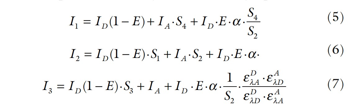
flow-cytometric-fret-analysis-of-protein-interaction-protocol-5-7

Here, E is the FRET efficiency, I_D and I_A are the unquenched donor and direct acceptor fluorescence intensities, and e denotes the molar absorption coefficient of the donor (D) or acceptor (A) labeled in the upper index, at the donor (λ_D) or acceptor (λ_A) excitation wavelengths.

7. From the above system of equations, E can be calculated as follows:

flow-cytometric-fret-analysis-of-protein-interaction-protocol-8

8. In most cases, the above equation can be simplified by neglecting some of the constants. For example, S3, S4, and the absorption ratio are negligible for the Cy3–Cy5 donor–acceptor pair measured on a FACSCalibur. In this case, the equation can be rewritten in the following form:

flow-cytometric-fret-analysis-of-protein-interaction-protocol-9

9. During data analysis, it is advised to follow a general scheme. First, one needs to determine the mean background intensities and the autofluorescence correction factors. Then calculate the alpha factor and spectral overspill parameters (Sfactors) from the acceptor- and donor-labeled samples. With these parameters in hand, now the energy transfer efficiency can be determined on a cell-by-cell basis.

FCET with Cell-by-Cell Autofluorescence Correction

If the fluorescence intensity of the samples is comparable to autofluorescence, subtraction of a constant autofluorescence value can result in serious errors in the calculation. In addition to analysis steps described under Subheading 3.4, perform the following steps:

From unlabeled sample 1, determine factors B₁, B₂, and B₃ characterizing the spillover of autofluorescence from the autofluorescence channel to the donor, FRET, and acceptor channels, respectively.

flow-cytometric-fret-analysis-of-protein-interaction-protocol-10

2. For the donor-labeled sample used for calculating S₁ and S₃, also determine factor S5 characterizing the spectral spillover of donor fluorescence from the donor channel to the autofluorescence channel:

flow-cytometric-fret-analysis-of-protein-interaction-protocol-11

3. For the acceptor-labeled sample used for assessing S₂ and S₄, also determine factor S₆ characterizing the spectral spillover of acceptor fluorescence from the acceptor channel to the autofluorescence channel:

flow-cytometric-fret-analysis-of-protein-interaction-protocol-12

4. The fluorescence intensities of the double-labeled samples can be expressed by the following set of equations:

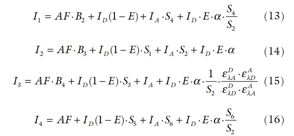
flow-cytometric-fret-analysis-of-protein-interaction-protocol-13-16

where AF denotes the autofluorescence intensity of single cells.

5. The above set can be converted to a system of linear equations by substituting the variable IDXE by X.

flow-cytometric-fret-analysis-of-protein-interaction-protocol-17-20

6. The solution of this equation system in general can be expressed as

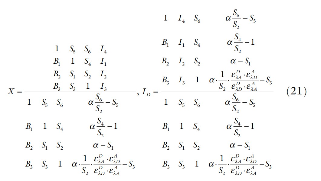
flow-cytometric-fret-analysis-of-protein-interaction-protocol-21

7. From this, the FRET efficiency E can be calculated according to the following equation:

flow-cytometric-fret-analysis-of-protein-interaction-protocol-22

When using the Cy3–Cy5, and AlexaFluor546–AlexaFluor 647 FRET pairs, and assigning the FL1 channel of a FACSCalibur to measure the cellular autofluorescence, the S3, S4, and S6 factors and the absorption ratio become negligible and the equation takes a much simpler form that can be used for calculating E as a new cellular parameter in the list mode file (see Note 13):

flow-cytometric-fret-analysis-of-protein-interaction-protocol-23

Interpretation of FCET Data

Although FRET can provide very useful information about molecular proximity and associations, it has its own limitations. The most serious drawback of FRET is that it has restricted capacity in determining absolute distances because FRET efficiency depends not only on the actual distance between the donor and acceptor, but also on their relative orientation. It is still quite good at determining relative distances, namely, whether the two labels are getting closer or farther upon a certain treatment/condition. Even when measuring relative distances, care must be taken to ensure that the orientation does not change between the two systems to be compared. Fluorophores attached to proteins via flexible linkers (such as a 6–12 carbon linker in the case of dyes or a few glycines in the case of fluorescent proteins) are relatively free to rotate, which allows for the donor and the acceptor to assume several spatial orientations during the excited-state lifetime of the donor (called dynamic averaging), which allows for optimal FRET measurements in complex biological systems. Conversely, rigid systems or changes of donor–acceptor orientation to positions less favoring FRET can lead to an underestimation of actual proximity. Thus, it is advisable to use alternative approaches in order to prove the reason for observed changes in FRET efficiency convincingly. For example, if fluorescent antibodies are used and if antibodies against different epitopes are available, it is advisable to test them as well.
Another problem is that FRET has very sharp distance dependence. Owing to this, it is difficult to measure relatively long distances because the rate of FRET gets very low. At the same time, energy transfer tends to occur on an all-or-none basis: if the donor and acceptor are within 1.63×R0 distance, energy transfer is detectable; if they are farther apart, energy is transferred with very little efficiency. Due to this sharp decrease, the absence of FRET is not a direct proof of the absence of molecular proximity between the epitopes investigated. Also, absence of FRET can be caused by steric hindrance even for neighboring molecules or protein domains. On the contrary, the presence of FRET to any appreciable extent above the experimental error of measurement is a strong evidence of molecular interactions.
Indirect immunofluorescent labeling strategies may be applied to FRET measurements if suitable fluorophore-conjugated mAbs are not available, or as an approach to enhance the specific fluorescence signal (see Note14). In such cases, special attention should be paid to the fact that the size of the antibody complexes used affects the measured FRET efficiency values. Application of a larger antibody complex causes a decrease in FRET efficiency due to the geometry of the antibody complexes, since when antibody or F(ab′) complexes become larger, the actual distance between the donor and acceptor fluorophores increases. FRET values cannot be compared directly to each other if they are obtained using different labeling strategies.
Another possibility for increasing the fluorescence signal is to use phycoerythrin (PE)- or allophycocyanine (APC)-labeled antibodies, since PE and APC have exceptional brightness. However, the size of these molecules is comparable to, or even greater than, that of whole antibodies. Due to steric limitations, the measurable FRET efficiency values can be low, at the border of detection limit. Nonetheless, it should be noted that even these low FRET efficiency values might have a biological meaning, since the accuracy of measurements is greatly improved owing to the high level of specific signals. Appropriate positive and negative controls can help make the decision whether the given molecules are associated or not on the basis of the measured FRET efficiency values.
When studying cells labeled with donor- and acceptor conjugated monoclonal antibodies, averaging is performed at different levels. The first averaging follows from the random conjugation of the fluorescent label. An additional averaging is brought about by the actual distribution of separation distances between the epitopes labeled with monoclonal antibodies. This multiple averaging, an inevitable consequence of the non-uniform stoichiometry, explains why the goals of FRET measurements are so uniquely different in the case of purified molecular systems on the one hand, and in the case of in situ labeled membrane or cytoplasmic molecules on the other hand. In the former case, FRET efficiency values can be converted into absolute distances, while in the latter, relative distances and their changes are investigated.
Calculation of distance relationships from energy transfer efficiencies is easy in the case of a single-donor/single-acceptor system if the localization and relative orientation of the fluorophores are known. If the FRET measurements are performed on the cell surface or inside the cell, many molecules might not be labeled at all; many could be single without a FRET pair, while others may be in smaller groups of heterooligomers, creating higher rates of FRET than expected from stand-alone pairs. A large number of epitopes binding the acceptor increases E simply by increasing the rate of FRET rather than actually meaning that the two epitopes investigated are closer to each other. If, in these cases, reversing the labeling still results in large E values, the proximity can be considered verified. However, if reversing the ratio of donor: acceptor to >1 makes FRET disappear, chances are that we have previously seen random colocalizations due to the high number of acceptors. One can use model calculations to predict the average distance of donors and acceptors, assuming random distribution, and compare the predictions of the calculations to the observed FRET efficiencies. Alternatively, the examination of the dependence of FRET on acceptor density and on the donor–acceptor ratio can help decide whether the examined proteins form clusters or are randomly distributed. However, the donor/acceptor ratios should be in the range of 0.1–10 if we want to obtain reliable FRET measurements. Outside this range, noise and data irreproducibility propagate unfavorably, rendering accurate FRET efficiency calculations impossible. It also needs to be noted that even random associations resulting from high expression levels of certain oncoproteins must not be regarded as biologically irrelevant.

Notes of Flow Cytometric FRET Analysis

Owing to the very large number of available fluorophores, it is impossible to present a thorough list of even the most widely used combinations. Excitation and emission spectra of molecules for donor–acceptor pair selection can be checked at one of the following web sites: Becton-Dickinson Fluorescence Spectrum Viewer, and Invitrogen-Molecular Probes Spectrum Collection. The number of available GFP variants has exploded in recent years. A paper to aid the selection of the optimal GFP variant has been published by the Tsien Laboratory. A detailed characterization of classical GFP variants for FRET experiments is also available. Recent developments are explored in refs.
Red-emitting fluorescent proteins are known to mature incompletely and, therefore, in tandem chimeric constructs where both donor and acceptor are in the same molecule, one cannot expect a 1:1 ratio for them; in fact, the average ratio will change from cell to cell. Furthermore, due to the incomplete maturation, exact proximity measurements cannot be performed reliably.
HEPES buffer (125 mM NaCl, 5 mM KCl, 20 mM HEPES, 1 mM CaCl₂, and 1.5 mM MgSO₄, pH 7.2) can also be used throughout instead of PBS, both for extra- and intracellular labeling.
Instead of 0.1% Triton X-100, 0.1% (w/v) saponin can be used. The saponin stock solution (20% w/v in dH₂O) should be stored frozen. Optimizing the signal and minimizing background for intracellular labeling are a must, but are beyond the scope of this chapter.
At least one donor-only and one acceptor-only sample are needed for spillage factors, and the same epitope labeled once with donor and once with acceptor is needed for calculating the α factor. It is a good approach, however, to prepare all the samples for obtaining independent determinations.
One needs to determine labeling intensity as a function of time after trypsinization for the particular proteins examined.
Time of labeling should also be optimized previously. Usually, incubation beyond 10 min does not increase labeling intensity by more than 10%.
The excitation and emission wavelengths for this channel I₄ are to be chosen such that the donor and acceptor fluorophores will not contribute considerably to the fluorescence intensity measured here. The main point is to obtain a fluorescence signature which is measured independent of the donor and acceptor channels (i.e., at least the excitation or the emission wavelength should differ from those of other detection channels), but can be used for calculating the contribution of cellular autofluorescence to these channels. There are alternatives to the arrangement proposed here, but this example is the one applicable to most commercial flow cytometers.
There is always one additional control to make, and that is to check for competition of the antibody carrying the acceptor with donor labeling. This should be done with the unlabeled antibody against the “acceptor” epitope, and any decrease of donor fluorescence caused by adding the unlabeled antibody should be attributed to competition rather than donor quenching due to FRET. Needless to say, competition between labeling antibodies is likely also a sign of molecular proximity, albeit not as readily quantitated as FRET.

In some rare cases, an antibody can increase the binding of another antibody. This enhancement can also lead to misinterpretation of FRET data. For example, if the acceptor-labeled antibody increases the binding of the donor-labeled antibody, the unquenched donor intensity of the donor+acceptor double-labeled sample is larger than that of the donor only sample, so the FRET calculated by comparing the donor intensity of the double-labeled sample and the donor-only sample will be underestimated. In some cases, the acceptor fluorescence may spill over to the donor channel, and the assumption that the background (i.e., non-donor) fluorescence intensity of the double-labeled sample is equal to the fluorescence intensity of the unlabeled sample does not hold. In such a case, a sample labeled by the acceptor-conjugated antibody and the unlabeled antibody against the donor epitope (to correct for the competition between the two antibodies) is to be used for background subtraction. An equation taking acceptor spillover and competition effects into account can be written in the following form:

flow-cytometric-fret-analysis-of-protein-interaction-protocol-24

Here, I_{Blank_donor+Acceptor} and I_{Donor+Blank_acceptor denote}, respectively, the fluorescence intensities (measured in the donor channel) of the sample tagged with the unlabeled antibody against the donor epitope and the acceptor-conjugated antibody, and that of the sample tagged with the donor-conjugated antibody and the unlabeled antibody against the acceptor epitope.

10. Although the spectroscopic spillover factors S1 through S6 are not expected to show any cell-by-cell heterogeneity, their cell-by-cell determination also has certain advantages. Performing mathematical calculations with cells having low fluorescence intensity introduces a large error into the calculations. Omitting these cells from the determination of the S factors greatly increases the reliability of these calculations.

11. Factor α is necessary to relate the actual fluorescence emission by the sensitized acceptor measured in the acceptor channel to the fluorescence one could measure in the donor channel from the donor if the quanta that are transferred in FRET had been emitted by the donor. This proportionality factor relates to the Q quantum efficiencies of the acceptor (index A) and donor (index D), and the detection efficiencies h in the acceptor and donor channels for photons emitted by the acceptor and the donor, respectively:

flow-cytometric-fret-analysis-of-protein-interaction-protocol-25

However, for practical purposes, a is more easily determined by measuring the same number of excited donor and acceptor molecules, respectively, in the donor and acceptor channels and normalizing them to their molar absorption coefficients (see Eq. 4). In Eq. 4 for α, there is a contribution from the sample labeled only with acceptor excited at the donor wavelength. Usually, this fluorescence intensity is rather small, thus giving the main error source in the calculations. To decrease this error, a should be determined using a protein that is abundant in our cells and recalculated for the actual antibodies used in the experiment.

The fluorescence quantum yields of the dyes may depend on the type of antibody they are attached to and even on the labeling ratio L, thereby affecting the value of α. The α factor determined for a given donor–acceptor antibody pair can be used for other antibody pairs labeled with the same dyes, provided its value is corrected for the differences in the quantum yields:

flow-cytometric-fret-analysis-of-protein-interaction-protocol-26

Here, subscript "1" refers to the antibody pair for which a has been determined previously and subscript "2" refers to the new antibody pair. Of course, such a correction requires the determination of quantum yields for the other antibody pair.

12. As already pointed out, autofluorescence values that are high compared to the donor and acceptor intensities can seriously disperse the calculated FRET efficiency distributions. Therefore, it is advisable to decrease the autofluorescence level as much as possible. A straightforward way to achieve this is to use yellow or red fluorescent dyes, since cellular autofluorescence becomes progressively weaker in the red region of the visible spectrum.

13. The simplified Eq. (23) is tested for the particular filter setup.

14. Optimizing the sensitivity of FRET measurements is a formidable challenge. To make the measurable range of molecular interactions as large as possible, donor–acceptor dye pairs should be chosen with the maximal spectral overlap. However, this will increase the cross talk between detection channels. At the same time, the higher the amount of spectral spillover compared to the FRET signal proper, the lower the reliability of the experiment. Therefore, efforts have to be made to minimize spectral spillover. A prudent approach to optimize the choice of fluorophores and filters to reach a balance between these contradictory requirements results in the recognition that the normalized fluorescence of applied dyes is an even more important asset ameliorating the detection of FRET through improved signal-to-noise ratio, and, collectively, AlexaFluor546 with AlexaFluor647 appears to be the most favorable FCET pair in a typical biological system.

Reference