
Inquiry Basket
 Loading ......
Flow cytometry is a technology that presupposes the availability of samples comprising single-cell suspensions, since it interrogates the fluorescence and light scatter properties of these cells as they stream individually in liquid through foci of intense light sources. The flowering plants, at most growth stages, do not exist in the form of single-cell suspensions. Instead, the predominant form is the multicellular sporophyte, with characteristic organs (leaves, roots, flowers, etc.) within which the tissues comprise complex interspersions of different cell types. Multicellularity arises through the controlled division of cells within meristematic zones. In contrast to animal species, sporophytic plant cells are non-motile and move away from the meristems solely as a consequence of cell division and subsequent expansion of the daughter cells. These cells, which in general have different fates, remain physically associated as a consequence of the mechanism of cell division, which subdivides the mother cell asymmetrically within the context of a shared, cellulosic cell wall. Therefore, prior to using flow cytometry to analyze plant cells, methods to produce single-cell suspensions are required. This can be done by dissolving the cellulosic cell wall under hyperosmotic conditions, which releases wall-less cells, termed protoplasts. Protoplasts, being bound by a plasma membrane devoid of much of the mechanical resilience found in animal cells, are inherently fragile; furthermore, they are characteristically larger, and sometimes much larger, than the mammalian cells that were used for establishing the original design specifications of flow cytometers. This introduces a number of additional complications in the successful flow analysis and, particularly, sorting of plant protoplasts. Special cases in which natural single-cell suspensions of plants are encountered include pollen and the developing microspores.
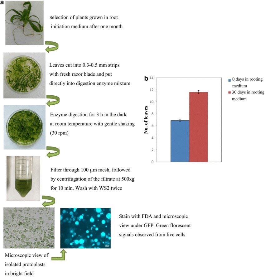 Figure 1. Schematic illustration of protoplast isolation. (Priyadarshani SVGN, et al.; 2018)
As an alternative approach for the flow analysis of plant systems, one can focus not on the examination of single cells, but on the examination of their subcellular contents. For this purpose, plant tissues and organs are converted into cell-free homogenates, and the constituents of the homogenates are subjected to flow analysis. In general, flow cytometers were not designed to accommodate this type of measurement, which is complicated by the fact that the objects of interest comprise an extreme minority of the total objects within the sample, and that the samples contain very high concentrations of objects detectable by the flow cytometer.
In employing flow cytometry and sorting with plant species, whether utilizing protoplasts or homogenates, a primary consideration is the purpose of the analysis. Considerable current interest exists in the use of flow-based methods for providing purified materials, protoplasts, or nuclei of specific cell types, as sources of transcripts for global gene expression profiling. This recognizes the need for single-cell resolution in deriving a genomic understanding of complex tissues and organs, in which different cell types are intricately interspersed.
This chapter, therefore, provides detailed information as to the best ways, using flow cytometry and sorting, to handle the complications presented by large particles and by crude homogenates, and to integrate these with genomic technologies aiming at characterization of global gene expression. I present specific details and helpful tips for successful operation of the cytometric instrumentation. My laboratory has experience working with the Coulter EPICS and Elite, the Cytomation MoFlo, the Becton Dickinson FACScan and LSR II, and the Accuri C6. The described methods are generally applicable to all of these instruments.
We first described flow analysis, sorting, and culture of plant protoplasts in 1984. In this work, we employed tobacco leaves as the source of protoplasts, since they are readily converted into protoplasts, and these protoplasts are particularly easy to take through tissue culture to regenerate cell walls and to induce organogenesis and thereby produce plants. Dissolution of the cell wall was achieved using mixtures of cellulases, hemicellulases, and pectinases, in the presence of an osmoticum, which serves to stabilize the plant plasma membrane under slightly hypertonic conditions. Since that time, we have described flow analysis and sorting of protoplasts from maize leaves and Arabidopsisroots, and these methods are applicable to Arabidopsis aerial tissues and leaves. Reports of the diameters of Arabidopsis protoplasts vary according to tissue and cell type: 10–20 mm for root protoplasts, around 30–50 mm for protoplasts prepared from well-expanded leaf tissues, and 10–20 mm for protoplasts prepared from aerial portions of plantlets grown on vertical agar plates.
Parameters available for flow analysis of protoplasts include the standard forward angle and 90° light scatter signals, as well as any fluorescence emission signals produced either from endogenous or from introduced fluorochromes such as the Green Fluorescent Protein (GFP). The shapes of the pulse waveforms over time can also be employed, for example, pulse width time-of-flight as a measure of cell size, but this has not found widespread use.
A prerequisite to the use of flow sorting for purification of specific cell types is a method to tag these cells which provides a fluorescent signal that can be detected by the cytometer. Particularly productive has been transgenic expression of members of the family of Fluorescent Proteins, of which the Green Fluorescent Protein (GFP) of Aequorea victoria is the archetype. The FP family now constitutes a large number of different proteins isolated from marine organisms, complemented by a large and ever-increasing number of sequence variants of these proteins.
As observed with other organisms, FPs can be readily expressed in plants and, with caveats, transgenic FP expression appears to be generally non-toxic within plants. FPs can be targeted to essentially all subcellular locations, using translational fusions to topogenic motifs or even entire proteins for this purpose. Caveats concerning the effects of excessive levels of expression and associated with mis-targeting should be noted. Targeting to subcellular organelles such as the nucleus provides increased signal-to-noise ratio, since background autofluorescence is generally dispersed throughout the cytoplasm. This advantage in sensitivity does not translate to flow cytometry when the fluorescence of the entire cell is quantified, but is a factor when analysis of isolated nuclei within cell-free homogenates is done.
For use in flow cytometry and sorting, the type of light sources that are available, including spectral quality and quantity, must be considered. Most forms of GFP and YFP are efficiently excited using the commonly available argon laser line at 488 nm, with DsRed and other red FPs being reasonably well excited using the krypton laser line at 568 nm. CFP excitation is optimal at around 425 nm, but it can also be excited at 457 nm (using a tunable argon laser), at 407/413 nm (using a krypton laser), or at 405 nm (using solid state laser diodes). BFP and its derivatives, which are of low brightness, are not routinely employed as fluorescent transgenic reporters.
For higher plants, mesophyll and epidermal cells within leaves can be defined based on the presence or absence of chlorophyll, and protoplasts can be analyzed, flow sorted, and characterized, based on this parameter. Plant protoplasts can also be analyzed and sorted based on transient or transgenic expression of GFP, as can nuclei. Combined flow analysis and sorting of GFP and RFP has also been recently reported. Cell type-specific FP expression involves the production of transgenic plants containing constructions in which the FP coding sequence is placed under the transcriptional control of specific promoters. Promoter/ enhancer trap methodologies can also provide transgenic plant lines within which selected subsets of cells are highlighted by FP expression. Work toward flow sorting of protoplasts and nuclei based on accumulation of FPs within specific cell types is ongoing at an increasing number of laboratories.
Plant protoplasts, in general, are heterogeneous in size and their diameters can be large in comparison to that of the flow tips with which flow cytometric instrumentation are conventionally equipped. Diameters, for example, frequently exceed 20–30 mm and are sometimes much larger, and flow analysis and sorting using standard flow tips (50–70 mm diameter) becomes impossible; for successful sorting, flow tips having diameters in the range of 100–200 mm may be needed. The applicable laws of physics impose constraints on the higher limits of actuation frequencies of the piezo drive responsible for synchronizing droplet production, which in turn limits the absolute rate of sorting. For this reason, sorting of nuclei, always having smaller diameters than protoplasts and hence allowing the use of smaller flow tips and resulting in higher sorting rates, may be advantageous in specific situations.
Flow cytometers conventionally employ light scatter signals to trigger the cycle of detection initiated when a particle enters the region of illumination. This is done for the simple reason that all particles, whether cells or of subcellular origin, scatter light; typically only a subset of these particles is fluorescent. Flow cytometric measurements involving mammalian cell suspensions benefit from the observation that most of the objects within the suspensions are those of interest (i.e., are cells). When employing plant homogenates for flow cytometric analysis, a very different situation pertains: the objects of interest comprise a small, and sometimes very small, minority of the light-scattering objects (i.e., debris) in the sample. A popular, important, and widely employed example is the measurement of nuclear DNA contents within plant tissue homogenates using DNA-specific fluorescent staining methods. The avalanche of light-scattering signals resulting from subcellular debris can obscure the detection of the objects of interest. Adjustment of discriminator settings to eliminate the contribution of this debris presupposes a knowledge of the light-scattering properties of the nuclei which, for novel samples, may not be a valid assumption. Further complications are introduced by the fact that the subcellular organelles themselves can exhibit autofluorescence, chloroplasts being a prime example. Employing protoplasts, rather than homogenates, may not completely forestall the problem of debris; for example, leaf mesophyll protoplasts contain large numbers of chloroplasts and the breakage of even a minor proportion of these protoplasts results in a considerable excess of chloroplasts over protoplasts within the cellular suspension. For this reason, use of isopycnic gradient flotation for protoplast purification is strongly recommended prior to flow analysis and sorting.
Although modern flow sorters can usefully operate at sort rates of around 40,000/s, the rate of recovery of specific cells is limited by the proportion of cells within the target tissue, the degree of enrichment/purification specified for the sort operation, and the size of the cells (which serves to define the upper sort rate). The total RNA content of eukaryotic cells is a function of nuclear DNA content, and varies also according to organism, species, tissue type, and developmental stage; typical values are ~1–100 pg of total RNA. Global transcriptional profiling generally employs one of two analytical platforms: DNA microarrays or, of increasing popularity, Next Generation DNA sequencing. For both platforms, microgram amounts of input target (targets being defined as the uncharacterized transcript-derived sample) are required. Target amplification techniques are, therefore, essential for studies integrating flow sorting with transcript analysis. Although amplification by a factor of 107 to 108 may appear daunting, commercial kits have been developed that are both robust and reproducible. In this chapter, we provide a description of methods that provide sufficient target for transcriptional profiling, down to the level of single sorted cells.
General Information and Precautions. Always wear a laboratory coat, disposable gloves, and a protective eyewear. Clean the working areas with 70% ethanol, before and after use. All chemicals are reagent grade, unless otherwise indicated. The following section lists specialty chemicals, kits, and equipment for the described applications and methods.
Microarray Hybridization
The following methods have been optimized for leaves and roots of A. thaliana, and are adapted. Seeds are sterilized and grown on vertical MS+ sucrose plates, as previously described.
1. Harvest roots or aerial parts of the plants by separating these tissues using a No. 22 scalpel, and then scraping them off the surface of the agar. Collect tissues on a Kimwipe moistened with diH2O and weigh them. Transfer to a 60×15 cm diameter plastic petri dish and add enzyme solution; proportions of 200 mg of tissue/5 mL enzyme digestion medium are recommended.
2. Segment the tissues in the enzyme solution using a single-edged razor blade, with the goal of producing tissue pieces that are ~1×1 mm (leaves) and 0.5×0.5 mm (roots). Transfer to an orbital shaker operating at 100 rpm and continue incubation for 60 min at room temperature.
3. After incubation, gently pipette the tissue fragments up and down ten times, using a disposable plastic transfer pipette with the end of the tip cut to produce a wider bore (~4 mm). Then filter the protoplast suspension through a 100-mm mesh cell strainer into a sterile polypropylene centrifuge tube.
4. Pellet protoplasts by centrifugation at 100×g for 3 min. All further manipulations are done on ice.
5. Remove the supernatant using a pipette and gently resuspend the protoplasts in 20.5% (w/v) sucrose dissolved in solution A, to a concentration of 3–10×105 protoplasts/mL. Transfer to a 10- or 50-mL tube as appropriate for the numbers of protoplasts. The lower (20.5% sucrose) phase should not occupy more than 50% of the volume of the tube. Gently overlay this phase with solution A, to fill the tube to about 90% of its total volume.
6. Centrifuge for 10 min at 500×g.
7. Collect protoplasts from the gradient interface using a transfer pipette and dilute with solution A prior to sorting. If necessary, the protoplasts can be concentrated by centrifugation at 100×g for 3 min. Measure protoplast diameters by light microscopy using a hemocytometer.
1. Excise plant materials (organs or tissues) and, if necessary, wash using diH2O. Transfer to a plastic petri dish (60×15 mm). Perform the remaining procedures on ice, and preferably in a walk-in cold room. It is convenient to place the petri dish on a prechilled ceramic tile embedded in an ice filled tray.
2. Add chopping buffer (2 mL per 0.5 g of fresh weight tissue represents convenient proportions for this size of petri dish). Chop the tissues using a new razor blade for 2–3 min.
3. Filter the homogenate through a 30-mm CellTrics® disposable filter to remove tissue debris.
4. Take an aliquot (0.5 mL) of the homogenate. If to be stained using PI, add this aliquot to a labeled tube containing 2.5 mL of a 10 mg/mL solution of DNAse-free RNAse A. Incubate on ice for 10 min. Add PI to a final concentration of 50 mg/ mL. If to be stained with DAPI, add the aliquot to a tube containing sufficient DAPI to give a final concentration of 20 mg/mL.
5. Incubate the stained samples on ice in darkness for 20 min prior to flow cytometric analysis.
1. Switch on the flow sorter and establish conditions for sorting using 10-mm Flow-Check™ Fluorospheres and settings appropriate for the specific instrument. Based on the size estimations obtained by hemocytometry under the light microscope, select a flow tip of appropriate diameter. Particles as large as 50% of the diameter of the flow tip can be successfully sorted and at high recovery rates. In the interests of establishing stable sorting conditions with minimal disturbance to protoplast integrity and recovery, it is often recommended that this diameter be at least threefold larger than the mean diameter of the protoplast population. This conflicts with issues concerning the amounts of sample generated during sorting, since droplet volume evidently increases rapidly with only slight increases in tip diameter. For the Cytomation Mo-Flo, and for Arabidopsis protoplasts prepared as described above, we employ a 70-mm flow tip and a sheath pressure of 40 PSI. This gives stable sorting, with a droplet delay of 20 at a piezo drive frequency of 60 kHz. These values should be considered as target ranges, since different instruments of the same type exhibit variation in responses.
2. For detection of fluorescence arising from chlorophyll autofluorescence and from GFP, employ 200 mW laser illumination at 488 nm.
3. Trigger events on side scatter and visualize the protoplasts using bivariate analysis of green fluorescence versus red fluorescence (the PMT screened by a 630/40 barrier filter), with beam splitting at 555 nm. While most flow cytometers are routinely configured to trigger using the forward-angle light scatter (FALS) signal, we find that, for plant samples, triggering based on 90° side scatter is a better option, since FALS detection generally appears to be noisier. This observation may be specific to the types of detectors employed for FALS acquisition. One must optimize the thresholding to allow the particles of interest to be visualized while excluding as much debris as possible. Draw an amorphous sort window to include the protoplast population. Perform sorting in "Enrichment Mode," with one to two droplets being sorted; this means that one droplet is always sorted, but if the desired event is in the leading or trailing half of the droplet, one more (preceding or trailing) droplet is also sorted. Sorting in Enrichment Mode provides the best combination of sample purity and sample recovery; the inevitable presence of subcellular debris, even for protoplast samples that are gradient purified, obviates sorting in single-droplet "Purity Mode" due to the triggering of too many sort aborts. Define the position of the sort region by first analyzing the negative control, and setting a lower boundary for a positive GFP signal. Next, adjust the left and right boundaries of the sort region to exclude non-GFP-positive protoplasts; determine the effects of sort window placement by sorting a few protoplasts onto a slide and examining them under a fluorescence microscope.
4. Validate instrument sort parameters by sorting 100 protoplasts onto a microscope slide, and examining and counting these under a light microscope.
5. Sort protoplasts into 0.6- or 1.5-mL centrifuge tubes. For isolation of RNA from populations of protoplasts, we sort protoplasts into tubes prefilled with 3.5 vol. of lysis buffer taken from the RNAqueous®-Micro Kit, assuming one final volume of sorted protoplasts. For sorting single protoplasts, prefill the tubes with 5 mL of the lysis buffer, step 1. Shake the tubes immediately to ensure that the sorted protoplast contacts the buffer.
6. Place the tubes on ice.
1. Perform the same procedure, step 1.
2. For combined detection of fluorescence arising from GFP fluorescence and from DAPI-stained nuclear DNA, employ laser illumination at 365 nm (40 mW) and 488 nm (200 mW).
3. Trigger events on side scatter and visualize the nuclei using bivariate analysis of blue–violet fluorescence (PMT screened by a 450/65 barrier filter) versus green fluorescence (PMT screened by a 530/40 bandpass barrier filter). Position a rectangular sort window to include the desired nuclear population. Perform sorting in enrichment mode, with one or two droplets being sorted per positive event.
The key to success relies on rapid denaturation of the RNA samples immediately following sorting. RNA is labile, and contamination by ubiquitous RNases is easy to achieve. Gloves should always be worn, all aqueous solutions should be made using DEPC-treated diH2O, and glassware should be autoclaved.
Two scenarios are described: the first involves sorting of "significan" numbers of protoplasts and nuclei, operationally defined as being 50,000–100,000; we typically recover around 100 ng of total RNA from 100,000 Arabidopsis nuclei. In this situation, macroscopic amounts of sorted liquids will accumulate as a function of sorting, so the issue is to dilute this with chaotropic RNA stabilizing buffers sufficiently to ensure that transcript degradation does not occur, which would otherwise introduce variability in consequent measurements of transcript abundance. The second scenario involves sorting of individual protoplasts. In this case, manipulations of single sorted objects represent the significant issue but, ultimately, success in detection and characterization of amplified transcripts, which experimentally turns out to be a stochastic process, provides valuable insight into the issue of noise in gene expression.
Preparation of RNA Targets from Populations of Sorted Protoplasts and Nuclei
Prepare RNA using the RNAqueous®-Micro Kit, which can conveniently accommodate an input sample volume of up to 0.1 mL. This procedure is executed exactly as described in the manufacturer's manual.
Preparation of RNA Targets from Single Sorted Protoplasts
This protocol merges information taken from the Applied Biosystems Technical Application Note and from Kurimoto et al.. The V1 and V3 primers are used for the purpose of first and second strand synthesis. Step 1 describes total RNA isolation. Steps 2–15 involve cDNA synthesis. Steps 16–20 describe the first round of cDNA amplification using PCR. Steps 21–26 provide a second round of PCR amplification. Steps 27 and 28 describe production of aRNA via in vitro synthesis from the amplified cDNA.
1. Prepare lysis buffer sufficient for 20 samples:
| μL | |
| GeneAmp® 10× PCR buffer II | 9 |
| 25 mM MgCl2 | 5.4 |
| 5% NP40 | 9 |
| 0.1 M DTT | 4.5 |
| V1 primer (10 ng/μL) | 1.8 |
| 2.5 mM dNTP mix | 1.8 |
| Prime RNase inhibitor (30 U/μL) | 0.8 |
| RNAguard RNase inhibitor (30 U/μL) | 0.9 |
| H2O | 56.8 |
| Total volume | 90 |
2. Add 5 mL of fresh lysis buffer to a 0.6-mL microfuge tube. Sort one protoplast into the tube, flick to mix, and centrifuge for 30 s.
3. Incubate at 70°C for 90 s. Centrifuge for 30 s and place on ice.
4. Prepare Reverse Transcription mix (sufficient for 12 samples):
| μL | |
| Superscript® III (200 U/μL) | 4 |
| Prime RNase inhibitor (30 U/μL) | 0.6 |
| T4 Gene 32 protein (5 mg/μL) | 1.4 |
5. Add 0.4 mL of this RT mix to each tube from step 3, mix by flicking tube, and centrifuge for 30 s.
6. Incubate at 50°C for 30 min, then inactivate the reaction by incubating for 15 min at 70°C. Centrifuge for 30 s and put on ice.
7. Prepare Exonuclease Mix (sufficient for 12 samples):
| μL | |
| 10× Exonuclease I buffer | 1.2 |
| H2O | 9.6 |
| Exonuclease I (5 U/μL) | 1.2 |
8. Add 1 mL of Exonuclease Mix to each tube, mix by flicking, and centrifuge for 30 s.
9. Incubate at 37°C for 30 min. Inactivate by incubation at 80°C for 25 min. Centrifuge for 30 s and put on ice.
10. Prepare poly(dA) addition mix (sufficient for 12 samples):
| μL | |
| 10× GeneAmp® PCR buffer II | 7.2 |
| 25 mM MgCl2 | 4.3 |
| 100 mM dATP | 2.1 |
| H2O | 52 |
| TdT (15 U/mL) | 3.6 |
| RNase H (10 U/mL) | 3.6 |
| Total | 72.8 |
11. Add 6 mL of poly(dA) addition mix to each tube, mix by flicking, and centrifuge in a microfuge for 30 s.
12. Incubate at 37°C for 15 min. Inactivate by incubating for 10 min at 70°C. Centrifuge in a microfuge for 30 s and put on ice.
13. Prepare Second Strand Synthesis Mixture (sufficient for ten samples):
| μL | |
| 10× Ex TaqTM buffer | 76 |
| dNTPs (2.5 mM) | 76 |
| V3 primer | 15.2 |
| H2O | 586 |
| Ex TaqTM Polymerase | 7.6 |
14. Add 76 mL to each tube, mix, and spin.
15. Perform one PCR cycle:
a) 95°C for 3 min
b) 50°C for 2 min
c) 72°C for 20 min
16. Centrifuge for 30 s and put on ice.
17. The next step involves PCR for 24 cycles for initial cDNA amplification. Prepare PCR amplification mix (sufficient for ten samples):
| μL | |
| 10× Ex TaqTM buffer | 76 |
| dNTPs (2.5 mM) | 76 |
| V1 primer | 15.2 |
| H2O | 586 |
| Ex TaqTM Polymerase | 7.6 |
18. Add 76 mL to each tube, mix, and spin. Divide total volumes between two tubes, providing two tubes for each reaction (each ~80 mL).
19. Perform PCR for 24 cycles:
a) 95°C for 3.5 min.
b) 67°C for 1 min.
c) 72°C for 3 min (with +6 s added per cycle, for another 23 cycles, to give a total of 24 cycles).
d) 72°C for 10 min.
20. Purify the cDNA using the QIAquick PCR Purification Kit according to the manufacturer's instructions. Use 30 mL of elution buffer for elution, as described by the manufacturer.
21. Employ the entire sample for electrophoresis using 2% agarose gel (in 0.5× TAE buffer; the gel occupies an area of ~5×10 cm and the volume is 30 mL; this accommodates at least ten lanes). Excise the band at around 500–2,000 bp as defined, using a 100-bp ladder; this may only be present in a minority of the lanes.
22. Purify the cDNA from gel using the QIAquick Gel Extraction Kit, according to the manufacturer's instructions. Use 30 mL of water for elution, as described by the manufacturer. Measure cDNA concentrations in the sample using a NanoDrop spectrophotometer. Typical concentrations are around 2–6 ng/mL, with total yields being around 50 ng/ sample.
23. cDNA reamplification. This next step provides sufficient amounts of cDNA for further use in target preparation for microarrays or for NextGen sequencing. Mix for one sample:
| μL | |
| 10× Ex TaqTM buffer | 5 |
| dNTPs (2.5 mM) | 5 |
| V3 primer | 1 |
| V1 primer | 1 |
| H2O+cDNA | 37.5 (usually this involves 5 mL of cDNA, with the remainder being water) |
| Ex TaqTM polymerase | 0.5 |
| Total | 50 |
24. Perform PCR for 20 cycles:
a) 95°C for 5.5 min.
b) 64°C for 1 min.
c) 72°C for 5 min 18 s.
d) 95°C for 30 s.
e) 67°C for 1 min.
f) 72°C for 5 min 24 s (+6 s for each subsequent cycle, for another six cycles).
g) 95°C for 30 s.
h) 67°C for 1 min.
i) 72°C 6 min.
25. This cycle is repeated ten times, the total number of cycles being 18.
26. Purify the cDNA with the QIAquick PCR Purification Kit, according to the manufacturer's instructions. Use 30 mL of elution buffer for elution.
27. Employ the entire product for 2% agarose gel electrophoresis in 0.5× TAE buffer. Excise the bands that appear around 500–2,000 bp. Purify the cDNA samples using the QIAquick Gel Extraction Kit according to the manufacturer's instructions. Employ 30 mL of water for elution. Measure cDNA concentrations using a NanoDrop. Typical concentrations should be ~100 ng/mL, with totals being ~2–3 mg per sample. These are sufficient for NextGen sequencing on any of the commercially available platforms.
28. In vitro transcription of cDNA to aRNA. This step is used to provide targets for microarray hybridization. Prepare Transcription Mix; all chemicals are part of the Amino Allyl MessageAmp™ II aRNA Amplification Kit (amounts are for one sample):
| μL | |
| cDNA | 16 |
| ATP, CTP, GTP | 12 |
| UTP | 2 |
| aaUTP | 2 |
| 10× T7 buffer | 4 |
| T7 Enzyme mix | 4 |
| Total volume | 40 |
29. Clean up aRNA according to the manufacturer's instructions.
Coupling to Cy-3 and Cy-5, and microarray hybridization are done using protocols developed in the Galbraith laboratory.
Preparation of Cy3 and Cy5 Monoreactive Dye
These dyes are supplied as five aliquots; the content of each tube is sufficient for at least four labeling reactions. Dissolve the entire contents of a single tube in 22 mL of DMSO by flicking the tube several times, and leaving at room temperature for at least 30 min protected from light. Centrifuge at 1,000×g for 30 s to collect the dye at the bottom of the tube. The dye is ready for immediate use, but can be stored at −20°C for up to 1 month. Always protect the dye from light by wrapping the tubes with aluminum foil.
Target Labeling
1. Dissolve the dried aRNA with 5 mL of 0.2 M NaHCO3 buffer by flicking the tube several times and leaving the tube at room temperature for at least 20 min.
2. Add 5 mL of the Cy3 or Cy5 solution to each tube, and mix by flicking the tube several times.
3. Spin the tubes at 1,000×g for 30 s, wrap in foil, and incubate at room temperature for 2 h.
4. Unincorporated dye is removed using an RNeasy MinElute Cleanup Kit, according the manufacturer's instructions.
Microarray Hybridization
The following procedure is that recommended for long oligonucleotide microarrays printed on aminosilane-coated microarray slides, and produced by our laboratory.
1. DNA probe immobilization can be done at any time prior to hybridization. Re-hydrate the slide over a 50°C water bath for 10 s.
a) Hold the slide with the label side down over the water vapor.
b) Watch spots carefully so that they do not over-hydrate and start to merge.
2. Dry the slide by placing on a 65°C heating block for 5 s. Remove and allow to cool for 1 min.
3. Repeat steps 1 and 2 four times. (The rehydration step is important to obtain uniform spots lacking a "doughnut" effect; however, if you feel uncomfortable with the rehydration step, proceed directly to UV cross-linking).
4. Cross-link the DNA to the slide surfaces by exposing the microarrays, in batches, array-side up, to 180 mJ UV irradiation using a commercial cross-linker.
5. Wash the slide in 1% SDS (prepared in sterile diH2 O) for 5 min at RT on a shaker, or agitate by hand. It is convenient to employ a slide carrier for these steps.
6. Remove SDS by dipping the slides ten times into sterile diH2O.
7. Immediately transfer the slides to 100% ethanol, dip five times, and then incubate for 3 min with shaking.
8. Spin dry slides by centrifugation. Centrifuge at no more than 200×g for 2–4 min (see Note 2).
a) Pack the bottom of a 50-mL plastic conical centrifuge tube with Kimwipes, occupying a packed volume of about 5 mL.
b) Using forceps, carefully place the slide into a tube.
c) Centrifuge at no more than 200×g for 2–4 min.
d) Repeat centrifugation if any liquid remains on the microarray surface.
9. Repeat ethanol wash if any streaks are observed on the microarray surface after step 8.
10. Store the slide in a lint-free, light-proof box at room temperature but at low humidity (use of a desiccator is recommended).
11. Prepare the following hybridization mix in a microfuge tube (see Note 3):
| 20× SSC | 6.0 mL |
| Western blocking reagent | 3.6 mL |
| 2% SDS | 2.4 mL |
| Labeled targets (volumes as from the clean-up step) | |
| H2O | to 60 mL |
12. Denature labeled target by incubating the tube at 65°C for 5 min.
13. Transfer the tube to ice immediately, or apply target onto the slides directly.
14. Rinse ArrayIt™ Hybridization Cassette with distilled water and dry thoroughly.
15. Make sure the flexible rubber gasket is seated evenly in the gasket channel.
16. Add 15 mL of water to the lower groove within the cassette chamber.
17. Insert the microarray (1″ × 3″ or 25 × 75 mm slide) into the cassette chamber, DNA side up.
18. Place the LifterSlip over the microarray slide.
19. Apply the denatured target sample slowly to the one end of the LifterSlip and let it spread across the microarray by capillary action.
20. Quickly place the clear plastic cassette lid on top of the cassette chamber.
21. Apply downward pressure and manually tighten the four sealing screws.
22. Check all the screws to confirm a tight seal.
23. Place the cassette into a hybridization oven pre-equilibrated at 55°C (see Note 4).
24. Allow the hybridization reaction to proceed for 8–12 h.
25. After hybridization, remove the cassette, loosen the four sealing screws, and remove lid.
26. Remove the microarray slide from the cassette chamber using forceps and place the slides into the washing buffer. This is most conveniently done using a slide holder.
27. Wash the microarray slides in the following solutions for 5 min each:
28. Washing is done by immersing the slides in a glass slide-staining jar containing the appropriate volume of wash buffer, followed by placing it on an orbital shaker at 60 rpm. Pre-heat the first wash solution and make sure the slides are completely immersed in wash buffer.
a) 2× SSC, 0.5% SDS at 55°C.
b) 0.5× SSC at room temperature.
c) 0.05× SSC at room temperature.
29. After completion of the washes, spin dry the slide as described in step 8.
30. Scan slide immediately, or store in a light-tight box at room temperature under dry conditions. Immediate scanning is recommended. However, we have observed that properly stored slides (light protected, dry, RT) retain fluorescent signals for up to a month. Some reports indicate that environmental pollutants (ozone) can drastically affect fluorescence, particularly that of Cy5.
31. Examine the scanned images immediately to determine the number of elements that are near zero or are saturated (for a 16-bit scanner, this represents a value of 65,400). The proportion of the elements at these extremes should be acceptably low, since information is lost in either case. It is preferable to rescan with altered gain settings on the scanner than to proceed with the analysis of images containing large proportions of zero or saturated elements. We have found that although the absolute value of the intensity values may be reduced by scanning a second or third time, the relative fluorescence distribution is preserved, so information is not lost. Scanning a second time at higher PMT/laser values can also be done to move low intensity elements higher within the dynamic range. The two intensity distributions (at low and high PMT/laser values) can then be merged to provide an increased combined dynamic range.
32. Save the image as a TIFF file, and implement appropriate data extraction and statistical analyses.
The amounts of target produced are sufficient for NextGen sequencing using Roche-454, Illumina Solexa, or Life Technologies SOLiD platforms.
References
Loading ......
