
Inquiry Basket
 Loading ......
Since its introduction more than 20 years ago, the ELISPOT assay has been widely used to measure IFN-γ production by individual antigen-specific T lymphocytes in a variety of disease settings, including cancer immunotherapy, HIV vaccine, infectious disease, and autoimmunity research. With such widespread use of the ELISPOT assay, it is often of interest to combine data across multiple laboratories or to compare these data formally or informally. This can be challenging on several levels as laboratories vary in their standard operating procedures resulting in different levels of variability across institutions. In addition, cellular assays are intrinsically complex and hence variability can be difficult to control even within one center. The variability is influenced by several steps in the process, including (1) the cell material that goes into the assay, (2) the materials, reagents, and protocol of the assay itself, (3) the hard- and software and chosen settings for spot acquisition, and finally (4) the rules and/ or tests applied to analyze and interpret the raw data. This chapter focuses on the variation of the results due to the use of different approaches to determine whether a given set of raw data, i.e., the # of spot-forming cells (SFCs)/PBMCs, is considered a positive antigen-specific T-cell response.
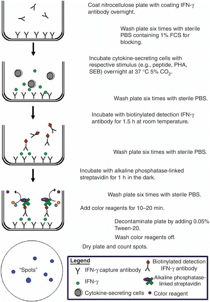 Figure 1. Schematic drawing of the principle of the Elispot assay. (Streeck H, et al.; 2009)
ELISPOT data are often first summarized in terms of the number of positive responders, hence various criteria to establish a positive response have been proposed, typically by comparing the data in the antigen-stimulated wells to the data in the negative-control wells. However, the various proposed methods can differ widely in their resulting positivity calls and no commonly accepted standard exists. Applying a common response determination criterion across laboratories would represent an important step toward reducing cross-laboratory variability.
This chapter reviews many of the commonly used methods for ELISPOT response determination and motivates the use of nonparametric statistical tests based on example data.
The data example considered is based on data from three consecutive interlaboratory testing projects organized by the Cancer Immunotherapy Immunoguiding Program (CIP). In these studies, 11, 13, and 16 laboratories (phases I, II, and III, respectively) quantified the number of CD8+ T cells specific for two model antigens with PBMC samples that were centrally prepared and then distributed to the participating laboratories. All participants used their preferred ELISPOT protocol, and therefore the datasets generated in these studies can be considered representative of results generated by a wide range of different protocols commonly applied within Europe. Each laboratory was asked to test in triplicate 18 preselected donors (5 in the phase I, 8 in the phase II, and 5 in the phase III) with two synthetic peptides (HLA-A*0201 restricted epitopes of CMV and influenza) as well as PBMC in medium alone for background determination. The selection of the donors was such that 21 donor/antigen combinations (6 in the first phase, 8 in the second phase, and 7 in the third phase) were expected to demonstrate a positive response with the remaining 15 donor/ antigen combinations not expected to demonstrate a positive response. Pretesting of potential donor samples for the proficiency panels was performed at two time points by two independent labs. Only samples from donors that had consistent results in all four performed experiments were selected for use in the proficiency panels.
The two principal approaches of determining a positive response in ELISPOT assay data are empirical and statistical.
The empirical approach typically employs a threshold for the difference between the mean spot counts in the antigen-stimulated experimental wells and those in the negative-control wells and/or an x-fold change between the means of the experimental and negative-control wells. These thresholds are meant to represent biological significance and may be laboratory-, procedure-, and operator-dependent. Ideally, empirical criteria should be based on an independent, blinded study of known positive and negative samples to determine operating characteristics, such as the true positive and true negative rates (i.e., sensitivity and specificity). It can be challenging to compare or combine responses across laboratories using different thresholds for positivity if the laboratories have diverse standards for establishing their respective criteria. Since empirical criteria are typically based on absolute or x-fold differences in mean responses, they therefore ignore the inherent variability in the data and also fail to detect extreme outliers. Mean responses that are derived from replicates that are highly variable provide much less-convincing evidence of a positive response than the means derived from replicates with very little variability, although the empirical rule would declare both to be positive responses. Conversely, differences that fall just below the threshold for positivity may be very convincing if the variability is extremely small, but would not be considered a positive response by the empirical criteria.
An additional drawback to the empirical approach is that the operating characteristics depend on how closely the datasets used to define the thresholds resemble the data to which the thresholds are applied. If the standard operating procedures of the assay change over time or if there are subtle shifts in the background of the assay over time, the thresholds may need to be redefined based on a new, blinded study of known positive and negative samples tested under the new conditions. Empirical criteria also do not offer uniform control of the false-positive rate when testing multiple antigens within the same sample, as is commonly the case.
The statistical approach employs a hypothesis test to formally compare the antigen-stimulated and negative-control well replicates. The quantitative responses (i.e., # SFC/PBMC) are then evaluated to determine whether the statistically significant differences are of scientific relevance, e.g., above the limit of detection of the assay. Various statistical tests for ELISPOT response determination have been recently proposed. The t-test is also commonly used, as many investigators are familiar with the test despite its strong assumptions in this setting. Nonparametric methods are better suited to settings, such as ELISPOT, where the sample sizes are small (e.g., triplicate wells) and the distribution of SFCs is unknown. The DFR(eq) criterion tests a null hypothesis of equal background, and experimental well means using a permutation test with Westfall-Young Stepdown max T adjustment for multiple testing across the different antigens or peptides considered. The DFR(2×) criterion tests a null hypothesis that the mean of the experimental wells is less than or equal to twice the mean of the background wells using a bootstrap test with the same multiplicity adjustment. As details of these methods can be found in the original references, this chapter focuses on the implementation of these methods and recommendations about which method is most applicable in a given setting. The DFR(eq) method is most appropriate in settings, where a significant difference in experimental and background well means is believed to indicate a positive response and a false-positive rate of 5% is acceptable. In settings, where one wants to control the falsepositive rate at a lower level and a larger significant mean difference is required to indicate a response (e.g., twofold over background), one might prefer DFR(2×). For example, a background-corrected mean of 20 per million PMBC is less striking when the mean background is 100 per million PBMC than when the mean background is 2 and the experimental mean is 22 per million PBMC. It is straightforward to modify the method to test for a different fold difference.
The DFR methods are based on nonparametric testing at the antigen/peptide pool level, and hence require a minimum number of replicates to ensure adequate power: at least three triplicates for experimental and negative-control wells or at least two experimental and four negative-control wells. Power and sensitivity increase with the number of replicate wells: three experimental wells and six negative control wells or four and four are the recommended minimum number of replicates based on simulation studies.
While response determination is an important element in the analysis of ELISPOT data, the quality of the data prior to response determination is also important to consider. Variability of the data is taken into account by the statistical test, but should also be considered as an element of quality control at the laboratory level prior to determining positive responses. In addition, the minimum level of response or limit of detection of the assay should be understood to aid in interpreting the scientific relevance of samples deemed positive by the response criteria.
To ensure adequate data quality, a variance filter for "extreme" outliers is suggested, whereby experimental replicates that do not pass the filter should be rerun or excluded. We recommend using the ratio of the variance to median + 1 as a measure of the variability of the spot counts within a replicate. The filter is designed to identify samples, where the majority of responses are low (hence, the median is small) but the variance is large due to an extreme outlier (see Note 2).
Data (see Note 3) may pass the proposed variance filter, be statistically significant yet the level of response be less than the lower limit of detection of the assay. The variance ratio is 0 and the sample is considered a positive response by both DFR(eq) and DFR(2×) due to the clear signal in the experimental wells yet the level of response may be too low to be considered a positive response. Before claiming that a statistical significant result is a positive response, the limit of detection of the ELISPOT assay should be taken into consideration. The international conference on harmonization of technical requirements for registration of pharmaceuticals for human use (ICH) produced a guideline, Q2R1, on the validation of analytic procedures. The limit of detection is defined there as the lowest amount of analyte in a sample that can be detected but not necessarily quantified as an exact value. The guideline describes three methods to estimate the limit of detection: visual evaluation, signal to noise, and response based on standard deviation and slope. The signal-to noise method best applies to the ELISPOT assay, where spot counts from the experimental wells are the signal and spot counts from the negative-control or background wells are the noise. A signal-to-noise ratio of 2:1 or 3:1 is generally considered acceptable for estimating the limit of detection. This guideline was applied to estimate the limit of detection across multiple laboratories following a broad range of representative ELISPOT protocols. As a typical ELISPOT protocol in these studies lead to a background of approximately 2 SFCs/100,000 PBMCs, the limit of detection for a laboratory showing average performance was estimated to be 4–6 SFCs/100,000 PBMCs. Hence, one might recommend that a response should not be considered positive if the mean of the experimental wells is less than the limit of detection even if the DFR methods declare a positive response. Laboratories may greatly differ in their limit of detection, however, and therefore the limit of detection should be established within each laboratory based on reliable datasets. This can then be used to guide the threshold for the minimum level of a positive response.
To demonstrate the large differences in results when using different methods to determine a response, we applied various methods to ELISPOT data described in the Materials section. Ten commonly used empirical rules and three statistical methods were applied to these data and the response detection rate and false-positive rates. A positive response was expected in 282 donor/antigen combinations and a negative response was expected in 196 such combinations.
The response detection rates and the false-positive rates can vary greatly depending on which response determination rule is used. With the empirical rules, the larger the required fold difference over background, the lower the overall response detection rate but the lower the false positive rate. Similarly, the larger the required minimum antigen spot count, the lower the response detection rate but the lower the false positive rate. These response detection rates are from a large group of laboratories with heterogeneous ELISPOT protocols, and therefore there is no prior experience as to which empirical rule would be the most appropriate to use. Examining the different empirical rules, it is not immediately clear which rule should be applied for response determination. All three of the statistical tests make a response determination using a p-value cutoff of 0.05. This implies that on average we would expect a 5% false-positive rate. In fact, the false-positive rate in this dataset is larger than 5% for both the t-test and DFR(eq) tests, but is smaller than 5% for the DFR(2×) test. When using the filters, the false-positive rates for all methods are less than 5%. The table illustrates how results can differ dramatically depending on which method is used for response determination although greater agreement between methods is seen when the filters are applied. The analysis underlines the need for standardization of the response determination process.
This chapter reviews objective methods to determine a positive response for ELISPOT assay data. The two main approaches, empirical and statistical, are reviewed and illustrated using an example dataset.
The main advantages of empirical criteria are that they are generally intuitive and easy to implement. The main drawbacks are that they do not account for the variability inherent in the data and they do not control the overall false-positive rate when multiple antigens are used, as is common practice. To appropriately justify the thresholds selected for empirical criteria, a laboratory would need to determine the sensitivity and specificity of these for a given assay protocol based on large representative datasets with known responder status (known positive and negative donors).
The main advantage of the statistical approach is that it can be applied with little prior knowledge of the operating characteristics of the assay protocol, therefore across a wide variety of settings, provided the assumptions of the statistical test are valid. In addition, statistical tests allow control of the false-positive rate as well as the overall false positive rate if multiple antigens are considered. The t-test requires parametric assumptions about the distribution of the data or a much larger sample size (rule of thumb: n > 30) than is practical for the number of replicate wells in the ELISPOT assay. A nonparametric test, such as used by the DFR(eq) or DFR(2×), is recommended. Both of these methods control the overall false-positive rate when testing multiple antigens and avoid parametric assumptions about the data.
In both empirical and statistical approaches, responses are determined by comparing experimental and negative-control well data. The background values for spot production can differ between donors and across time both within and across donors. Increases in the background spot counts influence the sensitivity of the method. Adding more replicate wells for both control and experimental conditions increases the power of the test. If resources are limited, increasing the number of negative-control wells results in appreciable gains, particularly when many antigens are tested since all antigens are compared to the same control wells within a donor. Six control wells are recommended whenever possible, with three experimental wells. Alternatively, four experimental and four control wells showed similar power to detect responses.
Prior to applying a statistical test, it is recommended that experimental replicates with large variance ratio, defined as the sample variance of the replicates divided by the median + 1, be excluded and/or rerun. The threshold for this should be based on laboratory experience. Replicates with a large variance ratio are likely to be errors and should not be considered reliable. If responses are expected to be large, a less-strict variance ratio may be used.
Responses that are declared positive by the statistical methods should be further examined for their relevance. For example, responses deemed positive may have net differences (i.e., mean experimental - mean negative control) that fall below the limit of detection of the assay although they are statistically significantly different. These should be interpreted with caution, thus some investigators might introduce a minimum threshold spot count below which results are considered negative.
In summary, there is solid statistical and empirical evidence to support the use of statistical hypothesis testing methods to determine ELISPOT response. Hence, a nonparametric method is recommended, such as the DFR(eq) or DFR(2×). The DFR(eq) method is preferred in settings, where a 5% false-positive rate is acceptable and one wants to detect low to moderate response magnitudes regardless of the level of background. The DFR(2×) method is appropriate in settings, where one wants more stringent control of the false-positive rate, e.g., 1%, and/or more stringent evidence of a fold difference in the means of the experimental and negative-control wells is more of interest than mere equality. Several user-friendly options are available to implement the recommended DFR statistical tests. A Web tool is also available at that address to upload a data file and run the code directly from the Web site; instructions are provided in the Notes. In addition, an Excel macro has also been developed to implement the statistical methods with Excel, available upon request.
Table 1. Example data for web tool at http://www.scharp.org/zoe/runDFR
| ID | Day | antigen | Well 1 | Well 2 | Well 3 | Well 4 | Well 5 | Well 6 |
| 14552 | 1 | Negctl | 9 | 4 | 9 | 2 | 6 | 7 |
| 14552 | 1 | Tyr | 27 | 25 | 21 | |||
| 14552 | 1 | Flu | 14 | 5 | 9 | |||
| 14559 | 1 | Negctl | 5 | 4 | 9 | 7 | 8 | 5 |
| 14559 | 1 | Tyr | 31 | 33 | 32 | |||
| 14559 | 1 | Flu | 12 | 7 | NA |
Once the data have been saved as a .csv file, point the browser to http://www.scharp.org/zoe/runDFR/ and enter the relevant information:
Number of antigens: 2.
Number of experimental wells: 3.
Number of control wells: 6.
Name of negative control: negctl.
Submit your .csv data file here (view an example): myfile.csv file created as described above.
Click on Run Me icon and wait for output to print on screen. The results may also be downloaded as a .csv file.
DFR(eq) positivity calls are listed in the "DFR(eq) response" column and DFR(2×) calls in the "DFR(2×) response" column. The corresponding p-values are listed in the respective adjusted p-value (adjp) columns.
Loading ......
